Ball & Beam Control - State space
코딩과 교육/전문코딩 2008. 7. 27. 18:08Ball & Beam Problem Using the State-space Design Method
The state-space representation of the ball and beam example is given below:
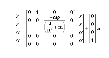
The design criteria for this problem are:
- Settling time less than 3 seconds
- Overshoot less than 5%
If you are interested in running an animation of this example based on the control techniques used in the state-space tutorial please go to the Ball & Beam Animation Page after completing this tutorial.
Full-State Feedback Controller
We will design a controller for this physical system that utilizes full-state feedback control. A schematic of this type of system is shown below:
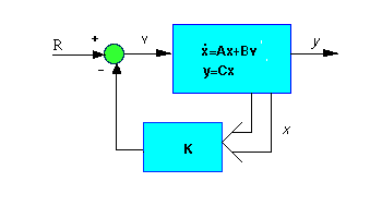
For our design we desire an overshoot of less than 5% which corresponds to a zeta of 0.7 (please refer to your textbook for the relationship between overshoot and damping ratio). On a root locus this criterion is represented as a 45 degree line emanating from the origin and extending out into the left-half plane. We want to place our poles on or beneath this line. Our next criterion is a settling time less than 3 seconds, which corresponds to a sigma = 4.6/Ts = 4.6/3 = 1.53, represented by a vertical line at -1.53 on the root locus. Anything beyond this line in the left-half plane is a suitable place for our poles. Therefore we will place our poles at -2+2i and -2-2i. We will place the other poles far to the left for now, so that they will not affect the response too much. To start with place them at -20 and -80. Now that we have our poles we can use Matlab to find the controller (K matrix) by using the place command. Copy the following code to an m-file to model the system and find the K matrix:
NOTE: Matlab commands from the control system toolbox are highlighted in red.
.....m = 0.111;
.....R = 0.015;
.....g = -9.8;
.....J = 9.99e-6;
.....H = -m*g/(J/(R^2)+m);
.....A=[0 1 0 0
........0 0 H 0
........0 0 0 1
........0 0 0 0];
.....B=[0;0;0;1];
.....C=[1 0 0 0];
.....D=[0];
.....p1=-2+2i;
.....p2=-2-2i;
.....p3=-20;
.....p4=-80;
.....K=place(A,B,[p1,p2,p3,p4])
Run your m-file and you should get the following output for the K matrix:
.....place: ndigits= 15
.....K =
..........1.0e+03 *
..........1.8286 1.0286 2.0080 0.1040
After adding the K matrix, the state space equations now become:

.....T = 0:0.01:5;
.....U = 0.25*ones(size(T));
.....[Y,X]=lsim(A-B*K,B,C,D,U,T);
.....plot(T,Y)
Run your m-file and you should get the following plot:
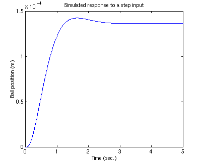
Reference Input
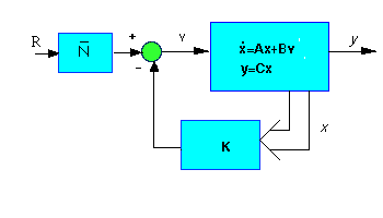
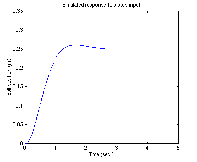
Now we want to get rid of the steady-state error. In contrast to the other design methods, where we feedback the output and compare it to the reference input to compute an error, with a full-state feedback controller we are feeding back both states. We need to compute what the steady-state value of the states should be, multiply that by the chosen gain K, and use a new value as our reference for computing the input. This can be done by adding a constant gain Nbar after the reference. The schematic below shows this relationship:
.....Nbar=rscale(A,B,C,D,K)
.....T = 0:0.01:5;
.....U = 0.25*ones(size(T));
.....[Y,X]=lsim(A-B*K,B*Nbar,C,D,U,T);
.....plot(T,Y)
Note: Non-standard Matlab commands used in this example are highlighted in green.
Your output should be:
.....place: ndigits= 15
.....Nbar =
..........1.8286e+03
Note: A design problem does not necessarily have a unique answer. Using this method (or any other) may result in many different compensators. For practice you may want to go back and try to change the pole positions to see how the system responds.


