Ball & Beam Control - Modeling
코딩과 교육/전문코딩 2008. 7. 25. 18:18VIA[CTM]
Problem Setup
A ball is placed on a beam, see figure below, where it is allowed to roll with 1 degree of freedom along the length of the beam. A lever arm is attached to the beam at one end and a servo gear at the other. As the servo gear turns by an angle theta, the lever changes the angle of the beam by alpha. When the angle is changed from the vertical position, gravity causes the ball to roll along the beam. A controller will be designed for this system so that the ball's position can be manipulated.
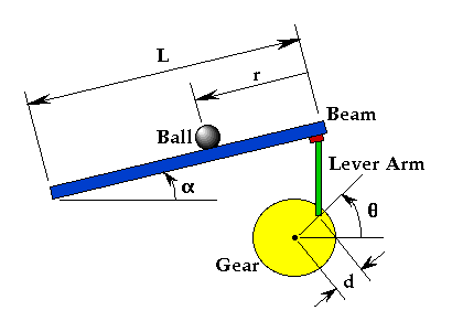
For this problem, we will assume that the ball rolls without slipping and friction between the beam and ball is negligible. The constants and variables for this example are defined as follows:
- M.........mass of the ball 0.11 kg
- R.........radius of the ball 0.015 m
- d.........lever arm offset 0.03 m
- g.........gravitational acceleration 9.8 m/s^2
- L.........length of the beam 1.0 m
- J.........ball's moment of inertia 9.99e-6 kgm^2
- r.........ball position coordinate
- alpha.....beam angle coordinate
- theta.....servo gear angle
The design criteria for this problem are:
- Settling time less than 3 seconds
- Overshoot less than 5%
System Equations
The Lagrangian equation of motion for the ball is given by the following:

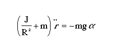

Substituting this into the previous equation, we get:

1. Transfer Function
Taking the Laplace transform of the equation above, the following equation is found:

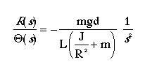
Rearranging we find the transfer function from the gear angle (theta(s)) to the ball position (R(s)).
2. State-Space
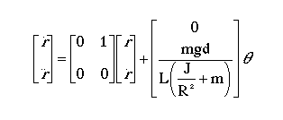
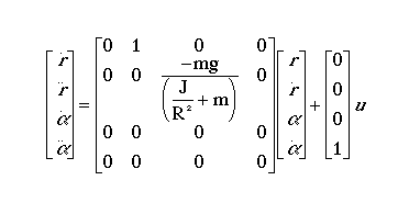
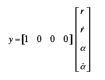
The linearized system equations can also be represented in state-space form. This can be done by selecting the ball's position (r) and velocity (rdot) as the state variables and the gear angle (theta) as the input. The state-space representation is shown below:
Matlab Representation and Open-Loop Response
1. Transfer Function
The transfer function found from the Laplace transform can be implemented in Matlab by inputting the numerator and denominator as vectors. To do this we must create an m-file and copy the following text into it:
.......m = 0.111;
.......R = 0.015;
.......g = -9.8;
.......L = 1.0;
.......d = 0.03;
.......J = 9.99e-6;
.......K = (m*g*d)/(L*(J/R^2+m)); %simplifies input
.......num = [-K];
.......den = [1 0 0];
.......printsys(num,den)
Your output should be:
.......num/den = 0.21 / ( s^2 )
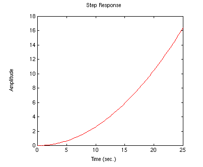
Now, we would like to observe the ball's response to a step input of 0.25 m. To do this you will need to add the following line to your m-file:
.......step(0.25*num,den)
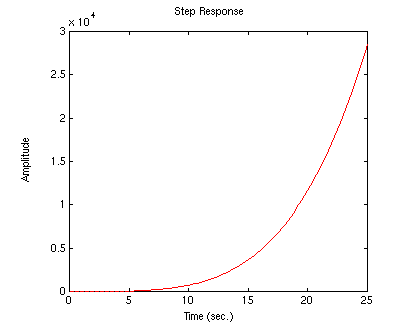
You should see the following plot showing the balls position as a function of time:
2. State-Space
The state-space equations can be represented in Matlab with the following commands (these equations are for the torque control model).
.......m = 0.111;
.......R = 0.015;
.......g = -9.8;
.......J = 9.99e-6;
.......H = -m*g/(J/(R^2)+m);
.......A=[0 1 0 0
....... 0 0 H 0
....... 0 0 0 1
....... 0 0 0 0];
.......B=[0;0;0;1];
.......C=[1 0 0 0];
.......D=[0];
The step response to a 0.25m desired position can be viewed by running the command below:
.......step(A,B*.25,C,D)
Your output should look like the following:
